Terraform Tips: Multiple Environments

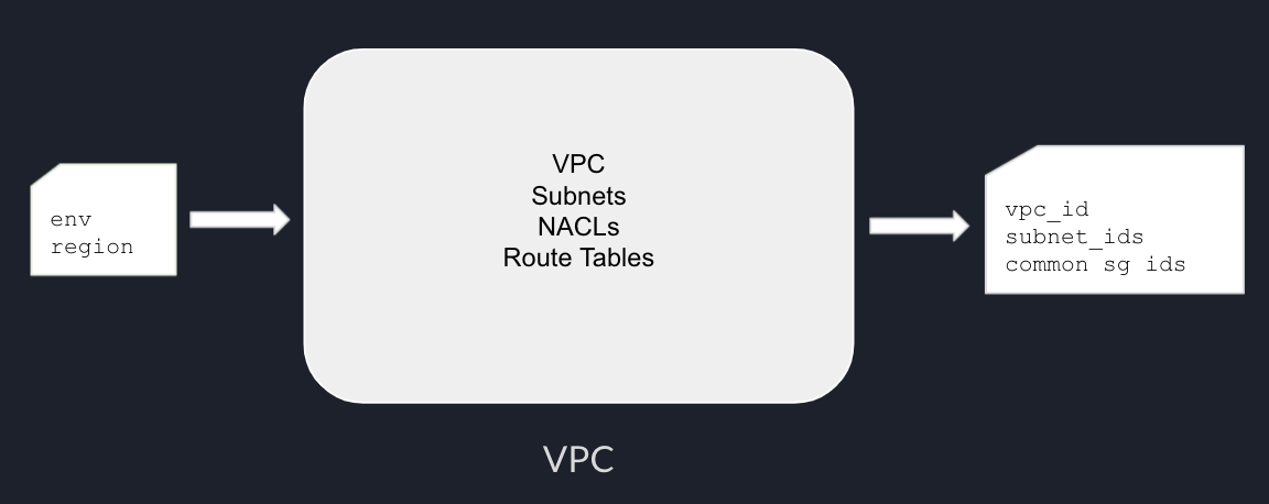
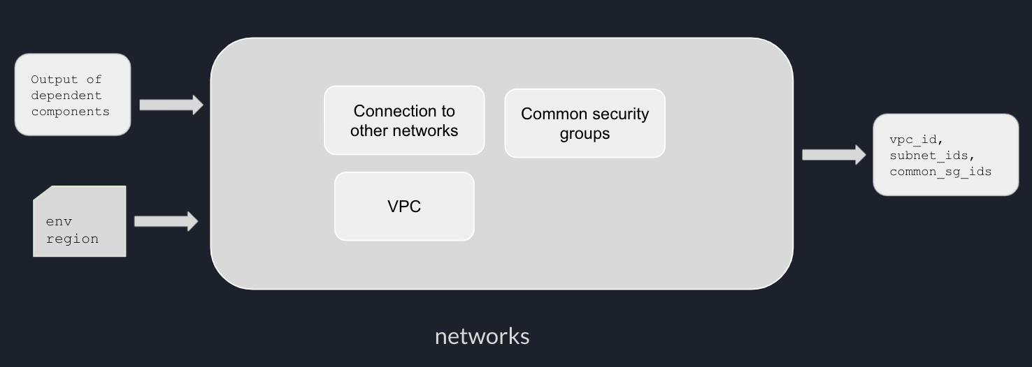
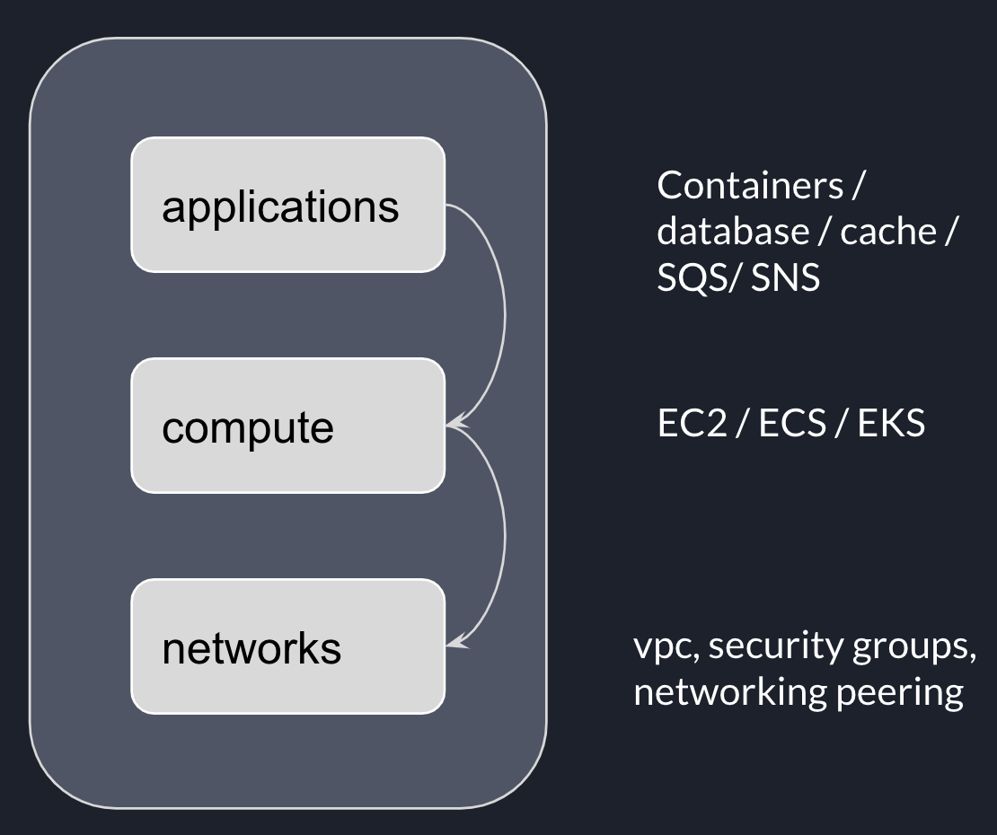
In last post, we explored the idea of layered infrastructure and the problem it was trying to solve.

One of the benefits of using Terraform to provision multiple environments is consistency. We can extract environment-specific configurations such as CIDR, instance size, as Terraform modules variables, and create a separate variable file for each environment.

In this post, we will talk about different options to provision multiple environments with terraform.

In a real-life infrastructure project, remote state store and state locking are widely adopted for ease of collaboration.

One backend, many terraform workspaces

I have seen some teams using terraform workspace to manage multiple environments. Many backends support workspace.

Let’s have a look at an example using S3 as the backend.

terraform {
  required_providers {
    aws = {
      source  = "hashicorp/aws"
      version = "~> 3.35.0"
    }
  }

  backend "s3" {
    bucket  = "my-app"
    key     = "00-network"
    region  = "ap-southeast-2"
    encrypt = "true"
    lock_table = "my-app"
  }
}

It is pretty straightforward to create multiple workspaces and switch into each workspace.

terraform workspace new dev
terraform workspace new test
terraform workspace new staging
terraform workspace new prod

terraform workspace select <workspace-name>

Each workspace’s states will be stored under a separate subfolder in the S3 bucket.

e.g.

s3://my-app/dev/00-network
s3://my-app/test/00-network
s3://my-app/staging/00-network

However, the downside is that both non-prod and prod environments’ states are stored in the same bucket. This makes it challenging to impose different levels of access control for prod and non-prod conditions.

If you stay in this industry long enough, you must have heard stories of serious consequences of “putting all eggs in one basket.”

One backend per environment

If using one backend for all environments is risky, how about configuring one backend per environment?

parameterise backend config

One way to configure individual backend for each environment is to parameterize backend config block. Let’s have a look at the backup configure of the following project structure:

├ components
│  ├ 01-networks
│       ├ terraform.tf  # backend and providers config
│       ├ main.tf
│       ├ variables.tf
│       └ outputs.tf
│
│  ├ 02-computing

terraform {
  required_providers {
    aws = {
      source  = "hashicorp/aws"
      version = "~> 3.35.0"
    }
  }

  backend "s3" {
    bucket  = "my-app-${env}"
    key     = "00-network"
    region  = "ap-southeast-2"
    encrypt = "true"
    lock_table = "my-app-${env}"
  }
}

Everything seems OK. However, when you run terraform init in the component, the following error tells the brutal truth.

Initializing the backend...
╷
│ Error: Variables not allowed
│
│   on terraform.tf line 10, in terraform:
│   10:     bucket         = "my-app-${env}"
│
│ Variables may not be used here.
╵

It turns out there is an open issue about supporting variables in terraform backend config block.

passing backend configure in CLI

terraform init supports partial configuration which allows passing dynamic or sensitive configurations. This seems a perfect solution for dynamically passing bucket names based on environment names.

We can create a wrapper script go for terraform init/plan/apply, which create backend config dynamically based on environment and pass as additional CLI argument.

Then we can structure our project as follows.

├ components
│  ├ 01-networks
│  │    ├ terraform.tf  # backend and providers config
│  │    ├ main.tf
│  │    ├ variables.tf
│  │    ├ outputs.tf
│  │    └ go
│  │
│  ├ 02-computing
│  │     ├ terraform.tf
│  │     ├ main.tf
│  │     ├ variables.tf
│  │     ├ outputs.tf
│  │     └ go
│  ├ 03-my-service
│  │     ├ ....
│
├ envs
│  ├ dev.tfvars
│  ├ test.tfvars
│  ├ staging.tfvars
│  └ prod.tfvars

Let’s take a closer look at the go script.

# go
_ACTION=$1
_ENV_NAME=$2

function init() {
  bucket="my-app-${_ENV_NAME}"
     key="01-networks/terraform.tfstate"
     dynamodb_table="my-app-${_ENV_NAME}"

     echo "+----------------------------------------------------------------------------------+"
     printf "| %-80s |\n" "Initialising Terraform with backend configuration:"
     printf "| %-80s |\n" "    Bucket:         $bucket"
     printf "| %-80s |\n" "    key:            $key"
     printf "| %-80s |\n" "    Dynamodb_table: $dynamodb_table"
     echo "+----------------------------------------------------------------------------------+"

     terraform init  \
         -backend=true  \
         --backend-config "bucket=$bucket" \
         --backend-config "key=$key" \
         --backend-config "region=ap-southeast-2" \
         --backend-config "dynamodb_table=$dynamodb_table" \
         --backend-config "encrypt=true"
}

function plan() {
  init
  terraform plan -out plan.out --var-file=$PROJECT_ROOT/envs/$_ENV_NAME.tfvars #use env specific var file
}

function plan() {
  init
  terraform apply plan.out
}

Then, we can run ./go plan <env> and ./go apply <env> to provision components for each environment with separate backed config.

Terraform Tips: Layered Infrastrucutre

Terraform have been a significant player in the infrastructure as code field. Since its first release in 2014, it has been widely used in the industry. Terraform finally reached 1.0 on 8 June 2021.

It is dead simple to provision and manages resources via terraform’s human-readable, declarative configuration language. However, you might only see the challenges when using it with anger in real-life projects. In this post, we’ll talk about the idea behind layered infrastructure; The problem it was trying to solve, and how to adapt it in your project.

Technically, we can provision a whole environment including networks, subnets, security groups, data stores, EC2 instances in one single terraform file. See the example below.

└── infra
    ├── prod
    │   └── main.tf
    ├── qa
    │   └── main.tf
    ├── dev
    │   └── main.tf
    └── stage
        └── main.tf

However, this would lead to a slow deployment process. To apply any resources changes, terraform would have to query and compare the state for each resource defined in main.tf.

We knew that the frequency of changes to different types of resources varies drastically; for example, the chance of changing the number of EC2 instances would be significantly higher than VPC CIDR. It would be a massive waste for terraform to compare hundreds of nearly unchanged resources to increase the instance number for an AutosScalingGroup.

If we use a remote state store, we can only apply any infrastructure changes to the environment one at a time.

There’s room for improvement. In a standard application deployment, we can classify these resources into layers such as application, compute and networks; the higher layer can depend on resources in lower layers.

Resources such as docker containers, data store, SNS topics, SQS queue, Lambda function are usually owned by an application. Resources such as EC2 instances, ECS or EKS clusters, providing computing capabilities, are usually shared across different applications.

Resources such as VPC, subnets, internet gateway, Network Address Translation (NAT) Gateway, network peering are essential to provision resources mentioned above. With these layered infrastructures, we can provision resources in different layers independently.

This is the idea of “layered infrastructure”, here is a layout of the project adopting layered infrastructure.

├ components       # components for an environment
│  ├ 00-iam           # bootstrap roles which will be used in higher layers
│  ├ 01-networks
│  ├ 02-computing
│  ├ 03-application
├ modules          # in-house terraform modules

As you can see from the layout, prepending number to component name makes it easy to understand their dependency.

Now let’s have a closer look at this layout. The layered infrastructure has three key concepts, module, component and environment.

Module

A Terraform module is a set of Terraform configuration files in a single directory intended to organise, encapsulate, and reuse configuration files, providing consistency and ensuring best practices. A terraform module usually has the following structure:

.
├── LICENSE
├── README.md
├── main.tf
├── variables.tf
└── outputs.tf    

For example, terraform-aws-vpc is a community module that can be used to provision VPC with subnets.

You can also maintain in-house terraform modules for shared codes within your organisation. Module

Component

An environment components groups multiple closely related modules or resources together. It can be provisioned independently within an environment. A component might depend on other components; Cyclic dependency must be avoided in component dependencies. A component usually has the following structure:

.
├── terraform.tf // backend configuration
├── provider.tf
├── main.tf
├── variables.tf
├── outputs.tf
└── go           // entry point for `terraform plan`, `terraform apply` and `terraform destroy`

Example of network components. Component

Environment

In the context of infrastructure as code, an environment is an isolated deployed instance of one or more components configured for a specific purpose, e.g. “dev”, “test”, “staging”, “production”.

All environments should have the same layout, with knot can be adjusted according to each environment. The only difference between environments should be captured in an environment-specific file tfvar. Let’s revisit the example project layout for an environment.

├ components          # components for an environment
│  ├ 00-iam           # bootstrap roles which will be used in higher layers
│  ├ 01-networks      # manage VPC, subnets, common security groups. output vpc/subnets/security group id.
│  ├ 02-computing     # manage computing resources into the vpc/subnets.
│  ├ 03-application   # manage application-specific resources 
├ modules             # in-house terraform modules

Environment

There are many benefits of adopting this approach, such as

  • Enables independent provisioning of each component (when the component’s output doesn’t change)
  • Fast deployment for the benefits of less state comparison.

Conclusion

We explored the problem layered infrastructure trying to solve; The benefits of this approach, and how to adapt it in your project.
This idea was inspired by Terraform Best Practices.

A jounery of performance tuning KafkaStream application

In this post, we’ll discuss our journey of tuning the performance of a few Kafka and KafkaStream application.

Principals

Divide and conquer Breaking down overall performance target into individual components have been proved works very efficient. In a distributed system that has a dozen services, There could be many bottlenecks, which might interfere with each other; It is extremely challenging to test the hypothesis in such a dynamic environment.

By define performance target for individual components and strategically tackling “low hanging fruit”, We were able to archive significant improvement in a short period.

Measurement

It is essential to measure the system before even tuning it. Having measurement in place helps the team understand the current and historical performance of the system.

Usually, the performance tuning requirements are described in one of the following formats:

  • The 99th percentile of API response time must not be larger than x milliseconds(latency).

  • The system should completely process messages in n` seconds (throughput).

By creating customised metrics that measure latency and throughput, and create a dashboard from collected metric data, We’re able to test the hypothesis at a swift pace.

Observibility

With the measurement capability built-in, we do observe significant latency during performance testing. However, without comprehensive insights into the system, it is challenging to locate the bottlenecks.

There’re two types of metrics that are essential to have to build meaningful insights into an application:

  • infrastructure metrics e.g. CPU utilisation, Memory utilisation, Network IO, Disk IO

  • application metrics e.g. JVM metrics, Kafka producer, consumer, Kafka stream metrics etc.

Collecting these metrics and create a comprehensive dashboard for an application give us a single place to identify the potential bottleneck.

App Dashboard

There’re many options for metric collection and aggregation. We use AppDynamic to collect and visualise these metrics, it has been beneficial to be able to have the ability to look at these metrics retrospectively after we changed a few parameters.

Also, Kafka exports a load of metrics via JMX, people might be overwhelmed when looking to them. We found this blog post from datadog is the best of explaining the meaning and indication of some key metrics.

KafkaStream App Tuning

Offheap memory usage

Compared to an application that only uses plain old Kafka producer and consumer, KafkaStream application requires more resources.

We noticed that our KafkaStream application’s memory usage constantly growing and eventually used up all available memory.

It turns out that this is not a memory leak. Rocks DB used a large portion of off-heap memory (non-heap memory), even JVM heap memory usage is stabilised around 400MB, the RSS (Resident set size) of this application process continually growing.

KafkaStream creates local state store which is optionally backed up to changelog topic for stateful operation (e.g. join, groupBy, etc.).

The following formula illustrates memory requirements for a stream application with default rocks DB settings.

one_rocks_db_memory_footprint = write_buffer_size_mb  * write_buffer_count + block_cache_size_mb
 
# default one_rocks_db_memory_footprint is 16MB * 3 + 50MB = 98MB

over_all_footprint_of_one_windowed_state_store  =  partition_number * segment_count * one_rocks_db_memory_footprint 

# default over_all_footprint_of_one_windowed_state_store is 12 * 3 * 98MB = 3528MB

There’re eight windowed joins in our application, the off-heap memory is 8 * 3528MB = 28224MB.

By providing a customised rocksdb configure, we can limit the off-heap memory to less than 4GB, provided that we haven’t observed performance degradation.

Minimise overall latency

There’re multiple consumer and producers in a KafkaStream application. Any misconfigured consumer/producer properties could contribute to the overall delay.

  1. Consumer commit.interval.ms

    This value allows us to make a trade-off between throughput and latency. A larger value increases system throughput but adds “artificial delays”. A smaller value will lead to more frequent consumer offset commits.

  2. Producer batch.size and linger.ms The default value of batch.size is 16KB, and average record size is 6KB, which means the producer need perform a send operation for every 2~3 messages, plus there is inevitable network latency between our application and Kafka Broker. By increasing batch.size to 1MB and set linger.ms to 50, we reduced the network latency overhead per message, and observed improvements on throughput and latency.

Stateful Operation and Change log restore process

One of my favourite feature of KafkaStream is the stateful operation without losing the ability of horizontal scaling.

However, we could be caught by some unexpected behaviours without using this operation cautiously.

Kafka Stream creates a local state store for each partition to perform the stateful operation, with the option of back up data to changelog topic.

If retention.ms is not specified, broker config log.retention.ms(default 7 days) will be used as a retention period of changelog topic.

Choosing the right window size, changelog topic retention period is essential for avoiding a lengthy change log restore process.

Further Readings

Tracking the root cause of a topic co-partition issue

When joining streams in Kafka Stream application, one critical prerequisite is that topics need to be co-partitioned.

In this post, I’ll share my experience of tracking down an issue of topics not fulfilling co-partition guarantee, when using DefaultPartitioner and confluent’s KafkaAvroSerializer in topic key.

Background

  • Service A producing events to topic A, with key K.
  • Service B producing events to topic B, with the same key K.
  • Service C joins events from both topics A and topic B and produce a calculated result to topic C, with the same key K.
  • All topics have the same number of partitions 10.
  • These topics key schema registration strategy is TopicNameStrategy.
  • key serializer is KafkaAvroSerializer.
  • All three services use DefaultParitioner in the producer.

The Issue

Service A and B produces records with key k1 to corresponded topics, When service C create two KafkaStream from topic A and B, and join them together; it complains that no matching record for key k1.

Let’s revisit the definition of Copartition Requirements.

One additional item I would like to add to this requirements is:

For the same key, the record should be on the same partition across these co-partitioned topics.

Service C complains that it can not find a matching record for key k1 as it considers only records from the same partition on both topics, while in reality,k1 was sent to partition 2 of topic A but partition 0 of topic B.

Even the configuration of topic A and B, service A, B and C meet all the requirements defined above, why is that?

Uncover the root cause

The following diagram demonstrates how the partition number calculated. partition process

Firstly KafkaProducer delegate to KafkaAvroSerializer to serialize an Avro object to a byte array, the serialized result includes schema id.

//org.apache.kafka.clients.producer.KafkaProducer#doSend

//In current context, keySerializer is an instance of KafkaAvroSerializer
serializedKey = keySerializer.serialize(record.topic(), record.headers(), record.key());

Secondly, the keySerializer talk to schema registry to resvole the schema Id for topic key and append it to serialized bytes.

//io.confluent.kafka.serializers.AbstractKafkaAvroSerializer#serializeImpl

id = schemaRegistry.getId(subject, new AvroSchema(schema)); //as we're using TopicNameStrategy, the subject is "A-key" or "B-key"
ByteArrayOutputStream out = new ByteArrayOutputStream();
out.write(MAGIC_BYTE);
out.write(ByteBuffer.allocate(idSize).putInt(id).array());

Thirdly, KafkaProducer hand the serialzation result to DefaultPartitioner to calculate partition number.

//org.apache.kafka.clients.producer.KafkaProducer#partition

partitioner.partition(record.topic(), record.key(), serializedKey, record.value(), serializedValue, cluster;

Lastly, DefaultPartitioner calculate parition number from serialized key bytes.

// org.apache.kafka.clients.producer.internals.DefaultPartitioner#partition

// hash the keyBytes to choose a partition
return Utils.toPositive(Utils.murmur2(keyBytes)) % numPartitions;

Root Cause

  • Key schema registration strategy is TopicNameStrategy, The same schema of K is registered with topic A and topic B separately; hence different schema Id is generated for topic A topic B.

  • When service A and service B serializing k1 , they append the different schema Id in the serialized bytes; Even though the Avro serialized value of k1 in two services are identical, the serialized key bytes are different.

  • DefaultParitioner calculates partition from serialized bytes, and yields different partition number in two services.

Solution

There’re two ways to address this problem; both have pros and cons.

  • Use other primitive type and Serde in topic key, e.g. StringSerializer, LongSerializer, etc.

The upside of this approach is co-partition is guaranteed as long as these requirements are met. The downside is losing the ability to evolve key schema. (who want to do this anyway?)

  • Use a customized partitioner

The upside of this approach is the ability to evolve key schema. The downside is additional complexity to services.

Conclusion

Using DefaultPartitioner and KafkaAvroSerializer in the topic key will make the topic fail to meet co-partition requirements.

Caveats

RecordNameStrategy won’t help in this case, as when there’s a need to upgrade the key schema, new schema id will be generated, which in turn generate different serialized bytes and yield different partition number. Even for the same key.

readable angular tests

In this post, I’ll provdes some tips to create readable angular test.

General Tips

Use describe or nested describe to structure specs

  • Use top level describe to describe a public function or a feature of the component to be tested.
  • Use nested describe to group specs which share the same context.Check the following example:
//top level describe
describe('#landing page', function() {
    //nested describe
    describe('logged in as admin', function() {
        beforeEach(function(){
            //context setup code for an admin user
        });
        it('should be able to see admin link', function() {});
        it('should be able to see greeting message', function() {});
    });
	describe('login as member', function() {
        beforeEach(function () {
            //context setup code for an memebr user
        });
        it('should not be able to see admin link', function() {});
        it('should be able to see greeting message', function() {});
	});
});

Put variable declaration close to usage.

It is quite common to see a bunch of local variables defined at the top of a spec then initialize them somewhere else in the code. It makes it super hard to understand the value and usage of those variables when going through the code.

Service Specs Tips

Put more business logic into Service.

Some services we created are just a very thin wrap of $http, Eg. :

angular
    .module('MyApp')
    .service('MyService', ['$http', 
    function ($http) {
        this.get = function (projectId, myId) {return $http.get('/projects/' + projectId + '/something/' + myId);};
    }]);

dead simple but is it worth to test it?

Encapsulating business logic into Service instead of Controller or Directive will lead to a higher test coverage of the code.

Directive Specs Tips

Directive is hard to test, here’re some tips:

Make directive as small as possible

One common mistake I observed is that directives have too much responsiblity.
Only have view/rendering related code should live in directive, any other business logic should be extracted into a service. If the “extra” code is related another view extract into another directive.

Limit the usage of $scope variables.

In most cases, a private variable is good enough. Compared to private variable, scope variables are public accessiable, which violate the encapsulation princaple. Also, scope variables are bound to directive lifecycle. check the following example.

angular.module('MyApp')
.controller('MyController', ['$scope', '$stateParams', 'MyService',
function ($scope, $stateParams, MyService) {
	var self = this;
	self.isAdmin = false;
	self.canCreateUser = false;
	self.myDomain = null;
	//...
	MyService.get($scope.myId).then(function(data){
	    self.myDomain = data;
	});
	//...
}
Simple template

Avoid bussiness logic in templates. Replace them with directive methods that express the intent of the logic, Eg. :

  //Before Refactor
  //directive
  $scope.isAdmin = ...;
  $scope.canCreateUser  = ...;
  $scope.isFriday = ...;

//template
<a ng-if="isOwner && canEditDocument && isFriday">click me</a>
//After refactor
//directive
$scope.isEditable = function(){
    return self.isAdmin && self.canCreateUser && self.isFriday
}

//template
<a ng-if="isEditable()">click me</a>
//Three scope variables were replaced by one scope function
Do not test directive template

Given we have made the template simple, we don’t need to test them. Testing directive methods(e.g. isEditable) is much easier to deal with doms in template, but provides enough confidence of quality.